Unless you've been living under a rock for the past couple of years, you would have heard and probably used Ai models like ChatGPT, Gemini or Stable Diffusion. They can write your exams, debug code and create images that look realistic. All these "Ai" models comes under a field called Deep Learning.
Deep Learning comes under Machine Learning which uses multilayered neural networks to do tasks such as classification, regression, etc.. These multilayered neural networks combined together is what we call as a "model". The goal is to create the best possible model which gives the most accurate and "best" results.
So, what do I mean by "best" results? The "best" models are those which have the "best" parameters. Think of parameters as tiny knobs inside the model. Finding the perfect combination of these knobs will create a "best" model. So, how does the model know which way to turn the knobs?
And, that's where the loss function comes in.
A loss function is like a guide for the model which tells it how well it is doing at turning those knobs. It measures how far off the model's predictions are from the actual answers.
If you liked my "knob" analogy, check out my project I did an year ago to explain myself about loss functions and to think like a model.
Maximum Likelihood
We usually think that given an input x, the model just
spits out an output y, kinda like y = f(x),
where f is the model.
And yeah, that's not entirely wrong, because, well, that's what it does in the end!
but there's more to it.
The model doesn't magically know given an input x,
the answer is y.
Instead what it does is, create a conditional probability distribution
Pr(y|x) over a range of possible outputs y given input x.
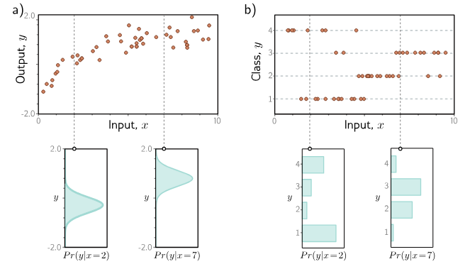
Figure: (a) Regression and (b) Classification
On the top plot, the orange dots show our data points. The bottom plot shows that the model outputs the probability distribution and and chooses the value as the output where the peak of the distribution comes. The width of the curve is uncertainity.
Source: Understanding Deep Learning: Chapter 5
On the top plot, the orange dots show our data points. The bottom plot shows that the model outputs the probability distribution and and chooses the value as the output where the peak of the distribution comes. The width of the curve is uncertainity.
Source: Understanding Deep Learning: Chapter 5
Well, now, you may have a doubt on how exactly a model f[x, ϕ] compute
a probability distribution.
The solution is really really simple.
What we actually do is, choose a parametric distribution Pr(y|θ)
defined on the output domain y.
So, for example, if the output domain is the set of real numbers,
we might choose univariate normal distribution, else, if the output domain
is a set of K distinct categories (Example: 'Cat', 'Dog', 'Bird', etc..),
we might choose the categorical distribution.
Then, we use the model to predict the parameters of that distribution.
So, in the case of univariate normal distribution, it is μ (mean) and σ2 (variance).
So, instead of computing the distribution itself, we now compute the
model parameters θ for each training example x.
The output y should have high probability given it's conditional
distribution Pr(y|θ).
Now, given I training examples, we have to choose the model
parameters ϕ that can maximize the combined probability.
$$ \begin{align*} \hat{\phi} &= \underset{\phi}{\operatorname{argmax}} \left[ \prod_{i=1}^{I} \operatorname{Pr}(\mathbf{y}_i | \mathbf{x}_i) \right] \\ &= \underset{\phi}{\operatorname{argmax}} \left[ \prod_{i=1}^{I} \operatorname{Pr}(\mathbf{y}_i | \boldsymbol{\theta}_i) \right] \\ &= \underset{\phi}{\operatorname{argmax}} \left[ \prod_{i=1}^{I} \operatorname{Pr}(\mathbf{y}_i | \mathbf{f}[\mathbf{x}_i; \phi]) \right] \end{align*} $$
The final term is called Maximum Likelihood Criterion.
Before going further, let me explain the terms again.
θ - This is the distribution parameters. So, if we have normal distribution,
it is μ (mean) and σ2 (variance).
ϕ - This is the model parameters which we are going to find to minimize the
loss.
x - Input sample.
y - Output observed.
I - The total number of training examples.
Now, If you are in the Machine Learning domain, you would have heard about
the term i.i.d (independent and identically distributed).
We assume our data are i.i.d, which means,
independent - We multiply all the training examples in the above because of
our independence assumption. We assume each and every sample is independent
of each other.
identically distributed - This means we assume all the training samples
in the current data comes from the same probability distribution.
The total likelihood for our whole dataset is the product of the individual likelihoods. There is just one problem here. Multiplying thousand of small probabilities together will create a ridiculously small number and can cause numerical underflow. So, we introduce log in the equation and convert the multiplcation to addition.
$$ \begin{align*} \hat{\phi} &= \underset{\phi}{\operatorname{argmax}} \left[ \prod_{i=1}^{I} \operatorname{Pr}(\mathbf{y}_i | \mathbf{f}[\mathbf{x}_i; \phi]) \right] \\ &= \underset{\phi}{\operatorname{argmax}} \left[ \log \left( \prod_{i=1}^{I} \operatorname{Pr}(\mathbf{y}_i | \mathbf{f}[\mathbf{x}_i; \phi]) \right) \right] \\ &= \underset{\phi}{\operatorname{argmax}} \left[ \sum_{i=1}^{I} \log \left[ \operatorname{Pr}(\mathbf{y}_i | \mathbf{f}[\mathbf{x}_i; \phi]) \right] \right] \end{align*} $$
So, why is this allowed? wouldn't it cause some harm?
Actually, no. The logarithm is a monotonically increasing function
which means if a > b, then, log(a) > log(b).
Because of this, the value of ϕ that maximizes the total likelihood
will also maximize the log-likelihood.
One final thing before we start to create our own loss function, whether it's Machine Learning or Business, we generally think of minimizing the loss. So, we convert the maximum log-likelihood criterion to a minimization problem by multiplying by minus one.
$$ \begin{align*} \hat{\phi} &= \underset{\phi}{\operatorname{argmin}} \left[ -\sum_{i=1}^{I} \log \left[ \operatorname{Pr}(\mathbf{y}_i | \mathbf{f}[\mathbf{x}_i; \phi]) \right] \right] \\ &= \underset{\phi}{\operatorname{argmin}} \left[ L[\phi] \right], \end{align*} $$
Now, we have the final loss function L.
Constructing our own loss functions
Now, that you have understood Maximum Likelihood Criterion. Creating your own loss functions is easy and just 4 step process:
-
Step 1: Choose a probability distribution
Pr(y|θ)that naturally fits the type of data that your model will be giving. For example, if you are predicting a continous value, pick normal distribution. If you are predicting discrete classes like 'Cat', 'Dog' or 'Bird', pick categorical distribution. - Step 2: Next, make the Machine Learning model f[x,ϕ] to predict the distribution parameters, θ. Note, here, we are not directly predicting final answer, y. So, for a given input x, the model's f[x,ϕ] output will be the parameters θ that define the probability distribution. For example, if the probability distribution is normal, you can make it to predict the mean (μ).
- Step 3: Next, we will train the model to find the model's parameters ϕ, by minimizing the loss function, which is the NLL. So, $$ \theta = f[\mathbf{x}, \phi] \quad \\ \\ \quad \operatorname{Pr}(\mathbf{y}|\theta) = \operatorname{Pr}(\mathbf{y}|f[\mathbf{x}, \phi]) \\ \\ \hat{\phi} = \underset{\phi}{\operatorname{argmin}} \left[ L[\phi] \right] = \underset{\phi}{\operatorname{argmin}} \left[ -\sum_{i=1}^{I} \log \left[ \operatorname{Pr}(\mathbf{y}_i | \mathbf{f}[\mathbf{x}_i; \phi]) \right] \right] $$
- Step 4: Now, the model is ready to make predictions on a new data. when we give it a new input x, we can simply return the value at the peak of the distribution. This is the model's single best guess.
That's it. You can now create a loss function for any of your problems. We will go over some examples below.
Example 1: Univarite Regression
In the univariate regression, we predict a single continuous number (y) from some input (x). Following the steps from above, Step 1: Choose a probability distribution. We are choosing a normal distribution here. It is defined by two parameters: mean (μ) and variance (σ2). Step 2: Make the Machine Learning model f[x,ϕ] to predict the distribution parameters. In this case, we will be predicting mean (μ).
Step 3: Choose a loss function based on NLL and train the Machine Learning
model to find the best model parameters ϕ on that loss function.
Here is a step by step process on how to do it:
This is the probability density function.
$$
\operatorname{Pr}(\mathbf{y}|\mu, \sigma^2) = \frac{1}{\sqrt{2\pi\sigma^2}} \exp \left[ -\frac{(\mathbf{y}-\mu)^2}{2\sigma^2} \right]
$$
Since, we are computing the mean (μ) here, so, μ = f[x,ϕ]
$$
\operatorname{Pr}(\mathbf{y}|\mathbf{f}[\mathbf{x}, \phi], \sigma^2) = \frac{1}{\sqrt{2\pi\sigma^2}} \exp \left[ -\frac{(\mathbf{y}-\mathbf{f}[\mathbf{x}, \phi])^2}{2\sigma^2} \right]
$$
The below is our NLL based on the normal distribution. This is what we
want to minimize.
$$
\begin{align*}
L[\phi] &= -\sum_{i=1}^{I} \log \left[ \operatorname{Pr}(\mathbf{y}_i | \mathbf{f}[\mathbf{x}_i, \phi], \sigma^2) \right] \\
&= -\sum_{i=1}^{I} \log \left[ \frac{1}{\sqrt{2\pi\sigma^2}} \exp \left[ -\frac{(\mathbf{y}_i - \mathbf{f}[\mathbf{x}_i, \phi])^2}{2\sigma^2} \right] \right]
\end{align*}
$$
Since, we are trying to find the best possible parameters ϕ that minimize
the loss function. The two terms below in step 2 and step 4 can be
removed because it doesn't depend on ϕ.
But, doesn't it change the location of the minimum? Yes! It absolutely
does and i will explain about it in the next section.
$$
\begin{align*}
\hat{\phi} &= \underset{\phi}{\operatorname{argmin}} \left[ -\sum_{i=1}^{I} \log \left[ \frac{1}{\sqrt{2\pi\sigma^2}} \exp \left[ -\frac{(\mathbf{y}_i - \mathbf{f}[\mathbf{x}_i, \phi])^2}{2\sigma^2} \right] \right] \right] \\
&= \underset{\phi}{\operatorname{argmin}} \left[ -\sum_{i=1}^{I} \left( \log \left( \frac{1}{\sqrt{2\pi\sigma^2}} \right) - \frac{(\mathbf{y}_i - \mathbf{f}[\mathbf{x}_i, \phi])^2}{2\sigma^2} \right) \right] \\
&= \underset{\phi}{\operatorname{argmin}} \left[ -\sum_{i=1}^{I} \left[ -\frac{(\mathbf{y}_i - \mathbf{f}[\mathbf{x}_i, \phi])^2}{2\sigma^2} \right] \right] \\
&= \underset{\phi}{\operatorname{argmin}} \left[ \sum_{i=1}^{I} \frac{(\mathbf{y}_i - \mathbf{f}[\mathbf{x}_i, \phi])^2}{2\sigma^2} \right] \\
&= \underset{\phi}{\operatorname{argmin}} \left[ \sum_{i=1}^{I} (\mathbf{y}_i - \mathbf{f}[\mathbf{x}_i, \phi])^2 \right]
\end{align*}
$$
So, the final result is something we already know!
It is the least squares loss function!
$$
L[\phi] = \sum_{i=1}^{I} (\mathbf{y}_i - \mathbf{f}[\mathbf{x}_i, \phi])^2.
$$
Step 4: Once the model is trained, its output for a new input x is the mean μ of the predicted Normal distribution. Since, the mean is the highest point of the bell curve, it's the most probable value and serves as our single best guess for the prediction.
Why are we ignoring the constant terms?
Consider these two functions: $$y = x^2$$ $$y = x^2 + 5$$
Let's look at their graphs:
As you can see, a constant can only shift the location of the minimum but
doesn't change the minimum itself.
The minimum is still 0 for both the graphs but the location the minimum
appears is different (0 and 5, respectively).
I hope you understood this part.
Why didn't we consider variance as another parameter?
If you have noticed above in the step 2, we ignored the variance as a distribution parameter and focused only on finding the mean (μ). We assumed the variance is constant on the whole data. If you have been in ML space for sometime, you might have heard the term homoscedasticity and heteroscedasticity. This is what homoscedastic mean. If we do not assume the variance is constant, then, it means the model is heteroscedastic.
So, how does the loss function change if the model is heteroscedastic? To model this, we can design a network with two outputs: one that predicts the mean (μ) and another that predicts the variance (σ2). Since, the variance is a positive term, we will pass it to a squaring function. $$ \begin{align*} \mu &= f_1[\mathbf{x}, \phi] \\ \\ \sigma^2 &= f_2[\mathbf{x}, \phi]^2, \\ \end{align*} $$ Thus, the final loss function is, $$ \hat{\phi} = \underset{\phi}{\operatorname{argmin}} \left[ -\sum_{i=1}^{I} \left[ \log \left( \frac{1}{\sqrt{2\pi f_2[\mathbf{x}_i, \phi]^2}} \right) - \frac{(\mathbf{y}_i - f_1[\mathbf{x}_i, \phi])^2}{2f_2[\mathbf{x}_i, \phi]^2} \right] \right] $$ So, If you have been using the least squares loss function and if your variance is not constant, then, your model is not good. That's the reason why one of the assumption of linear regression is homoscedasticity.
During the inference time, should we output mean or variance? The answer is obviously mean because it represents the peak of the bell curve. So, what does variance tells us? It tells us the uncertainity of the prediction.
Example 2: Multiclass Classification
The goal of multiclass classification is to assign an input to one of K
possible categories.
Let's say, you are trying to build a machine learning model that
classifies the idli into 'normal', 'rich' or 'luxury'.
Here, K=3 and the output y must be one of these three labels.


Generated with ImageGen
Step 1: Choose a distribution that can handle this. The perfect distribution for this is categorical distribution. It's defined by K parameters, which we'll call λ1,λ2,...,λK. Each parameter represents the probability of one specific category.
For our idli classifier,
- λ1=Pr(y=’normal’)
- λ2=Pr(y=’rich’)
- λ3=Pr(y=’luxury’)
Step 2: We will use a neural network f[x,ϕ], with K=3 outputs to compute these probabilities. But, there's one problem here, the output will be a raw, unconstrained numbers. What if the network output is like this: [0.8, 1.4, 2.5]? These are not probabilities because they aren't between 0 and 1, and they don't sum to 1.
But, to convert those raw outputs into probabilities, we will use the softmax function. The softmax function converts a tuple of K real numbers into a probability distribution of K possible outcomes. $$ \operatorname{softmax}(z)_k = \frac{e^{z_k}}{\sum_{j=1}^{K} e^{z_j}} $$ The likelihood that an input x has the label y=k is given by applying softmax to the network's output: $$ \operatorname{Pr}(\mathbf{y}=k|\mathbf{x}) = \operatorname{softmax}_k[\mathbf{f}[\mathbf{x}, \phi]] \\ $$
Step 3: We will use a loss function (NLL) here to train our Machine Learning model. This is also known as multiclass cross-entropy loss. $$ L[\phi] = -\sum_{i=1}^{I} \log \left[ \operatorname{softmax}_{y_i} \left[ \mathbf{f}[\mathbf{x}_i, \phi] \right] \right] \\ = -\sum_{i=1}^{I} \left( f_{y_i}[\mathbf{x}_i, \phi] - \log \left[ \sum_{k'=1}^{K} \exp \left[ f_{k'}[\mathbf{x}_i, \phi] \right] \right] \right) $$
Step 4: Once the model is trained, we give it a new idli image. It computes the probabilities for each class. To make a single "best guess," we simply choose the class with the highest probability.
 -> Model -> Luxury
Conclusion
And, that's how you create your own loss function for any type of usecases.